A normal probability plot, whether on probability paper or not, can help you decide whether a set of values are from a normal distribution. To make this determination, you must apply the probability of a normal distribution, which, if you were doing it by hand, is where probability paper comes in. While Microsoft Excel doesn't have an actual print layout for probability paper, there are adjustments you can make to a chart to simulate this format.
Step 1: Enter Data Set
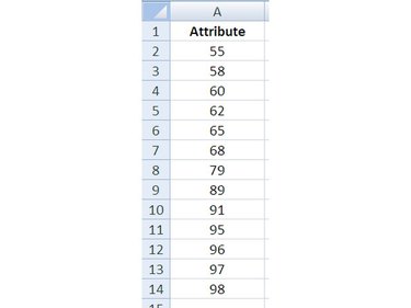
You have data that are the results of a small sampling and you want to know whether these data are from a normal distribution. Open Excel and enter the data on a worksheet.
Video of the Day
Step 2: Select the Data for Sorting
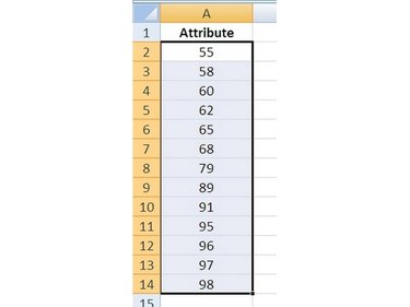
Select the data to be sorted by clicking into the cell with the first value (not the heading) and, while holding the mouse button down, move the mouse pointer down to the last value and release the button. The data cells should be shaded now, which means they are "selected."
Step 3: Sort the Data
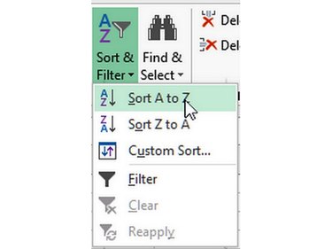
Click on the Home tab of the Excel Ribbon and click the Sort & Filter button to display its menu. Click on Sort A to Z (or low to high)to sort the data selected in the previous step.
Step 4: Number the Values
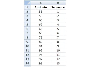
In a column adjacent to the data values, enter a sequence number, from top to bottom, for each of the values, numbering them from 1 to n, which in the example n = 13.
Step 5: Calculate the Mean
In a blank cell on the same worksheet as the data, enter the AVERAGE() function to compute the arithmetic mean of the data set:
=AVERAGE(First_Cell:Last_Cell)
First_Cell and Last_Cell refer to the beginning and ending cells of the data value range. In the example, the function statement is =AVERAGE(B2:B14).
Step 6: Calculate the Standard Deviation
Adjacent to the cell in which you calculated the mean, enter the STDEV() function to calculate the standard deviation of the values in the data set:
=STDEV(First_Cell:Last_Cell)
First_Cell and Last_Cell refer to the beginning and ending cells of the data value range. In the example, the function statement is =STDEV(B2:B14).
Step 7: Calculate the Cumulative Probabilities
Enter the NORMDIST() function to complete the cumulative probability of each value.
To complete the data needed to create a plot, the values need to be numbered in sequence, the associated z-value determined and the probability of each value along with a cumulative probability of all the values.
Video of the Day