How Do I Use a Letter to Represent a Value in Excel?

LOOKUP finds data in your worksheet so you can insert it in other cells.

Image Credit: Image courtesy Microsoft

Finding and using the same numbers repeatedly in Excel can be time-consuming, but there are a couple of ways to automate the process. The Name tool allows you to create shortcuts to enter data when you type an = sign followed by a letter. However, this doesn't work with C or R, which Excel reserves for its own shortcuts. If you need to use these letters, or want to work with existing data in your worksheet, use the LOOKUP function to create a formula to insert values when you want to use them.

Using a Name to Represent a Value

Video of the Day

Step 1

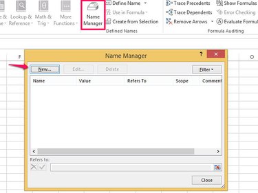
You can create, edit and delete names in Name Manager.

Image Credit: Image courtesy Microsoft

Open the Formulas tab. Select Name Manager and then New.

Video of the Day

Step 2

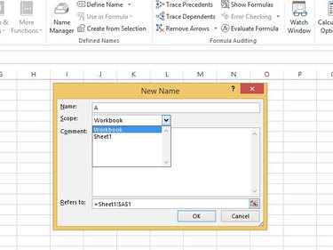
Excel applies names to the whole workbook by default.

Image Credit: Image courtesy Microsoft

Type A, or the letter you want to use as a value, in the Name box. Open the Scope drop-down menu and choose where you want to use the name. You can apply names to the whole workbook or to individual sheets.

Step 3

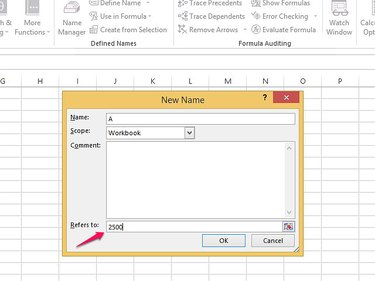
This example gives the letter A a value of 2,500.

Image Credit: Image courtesy Microsoft

Set the letter's value in the Refers To box. You can create a value from data in a cell in the worksheet or you can add your own number. By default, Excel puts a reference to the currently selected cell in the box. If this contains your value, keep the default. To use a different cell, select the reference in the box and click your new cell to make the switch. To set your own value, delete the cell reference and enter your number in the box. Select OK and then Close.

Step 4

Excel adds yellow tags to names.

Image Credit: Image courtesy Microsoft

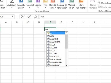
Select a blank cell in your worksheet to test that the name works. Type =A. You must use the = sign before the letter or the name won't work. You should see a drop-down menu with your name letter at the top. Select it or press the Enter key and the number you set as the value will appear in the cell.

Use LOOKUP to Create Letters and Values

Step 1

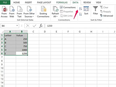
Make sure your values match the right letters.

Image Credit: Image courtesy Microsoft

Type Letter and Value as headers in columns A and B in your worksheet. Enter your letters in column A and their values in column B. If your data is not in ascending (lowest to highest) order, select it. Open the Data tab and use the Sort A to Z button to sort it.

Step 2

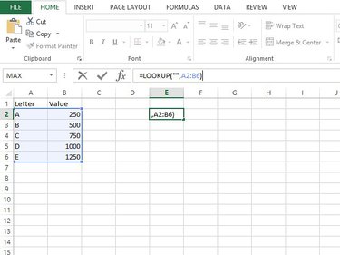
Excel automatically updates formulae when you change the data range.

Image Credit: Image courtesy Microsoft

Select an empty cell into which you want to add a letter value and type or paste =LOOKUP("",A2:B6) into the formula bar, where A2 and B6 define the range of data you want to search. Your data should have a line around it, showing the range in the formula. If this line doesn't contain all your letters and values, use the squares at the corners of the line to drag it over them.

Step 3

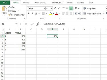
Copy and paste the formula to insert values when you need to use them.

Image Credit: Image courtesy Microsoft

Press the Enter key. The cell you've selected will contain #N/A because you haven't told Excel which letter to search for. Go to the formula in the bar, click between the quotation marks and type the letter C. Your formula should now read: =LOOKUP("C",A2:B6). Press Enter and the value of the letter. The value of C, 750, appears in your cell. To use values for another letter in your table, replace the C with the appropriate letter. For example, to insert the value of B in a cell, you would use =LOOKUP("B",A2:B6).