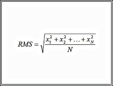
The Root Mean Square calculates the effective rate or measurement of a varying set of values. It is the square root of the average of the squared values in a data set. RMS is primarily used in physics and electrical engineering. One of the more common uses for an RMS calculation is comparing alternating current and direct current electricity.
For example, RMS is used to find the effective voltage (current) of an AC electrical wave. Because AC fluctuates, it's difficult to compare it to DC, which has a steady voltage. The RMS provides a positive average that can be used in the comparison.
Video of the Day
Video of the Day
Unfortunately, Excel doesn't include a standard function to calculate RMS. This means you'll have use one or more functions to calculate an it.
Step 1: Enter the Data Set
Enter your data values so that the raw data (measurement, test value, etc.) is located in a single column or row. Allow space adjacent to the data values to place the results of other calculations.
Step 2: Calculate the Squares
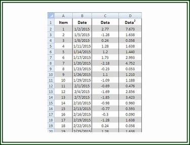
Calculate the square (x^2) for each of the values in your data set. Enter the formula =
Step 3: Average the Squares
Calculate the average of the individual squares. Below the last entry in the column containing the squares of the data set values, enter the formula =AVERAGE(First Cell:Last Cell). For example, =AVERAGE(D2:D30) calculates the mean (average) of the squares in the cells ranging from D2 to D30, inclusive.
Step 4: Calculate the Square Root of the Average
In an empty cell, enter the formula to calculate the square root of the average of the squares of the data. Enter the formula =SQRT(XN), where "XN" represents the location of the average calculated in the previous step. For example, =SQRT (D31) calculates the square root of the value in cell D31.
The value calculated in this step represents the RMS of the values in the data set.
Calculate the RMS with One Excel Formula
It is possible to calculate the RMS in a single formula using the original data values. The sequence of the steps, those of Steps 1 through 3, are as follows: calculate the square of each value, calculate the average of the squares and calculate the square root of the average.
The formula =SQRT((SUMSQ(First:Last)/COUNTA(First Cell:Last Cell))) uses the SUMSQ function to produce the sum of the squares of the values in the cell range. Then that number is divided by the number of cells containing data in the cell range specified (COUNTA). Finally, the square root of this value is calculated, which is the RMS.
For example, the formula =SQRT((SUMSQ(C2:C30)/COUNTA(A2:A30))) calculates the sum of the squares in the range C2 through C30, divides that sum by the number of entries in the range A2 through A30 that are not blank and then finds the square root of that value to produce the RMS.